How Do You Detect an Animal You've Never Seen?

If you have driven along Rifle Range Road recently, you might have noticed an animal crossing sign that lights up when something is near the road. During my internship, I worked on the part that decides when that sign should flash. A camera watches the forest edge while a model checks whether an animal is about to wander into traffic.

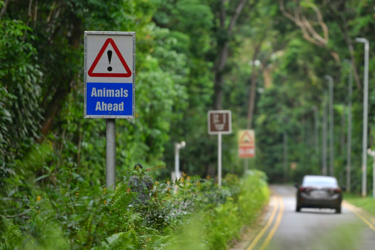
An animal crossing sign beside a forest-edge road in Singapore.

The job sounded easy enough at first. We would train a detector, point it at the road and use its output to trigger the sign. Then we ran into two requirements that pulled the system in different directions.

The sign has to react while the animal is still there, which rules out a slow API call or a dependency on the patchy connection beside a forest. At the same time, we cannot predict every species that might appear. Monkeys and deer are common enough to collect training data for, while animals such as civets, monitor lizards, snakes and pangolins turn up much less often.

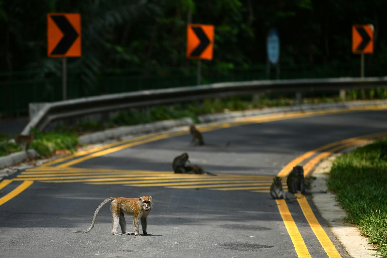
A fairly normal afternoon on a forest-edge road.

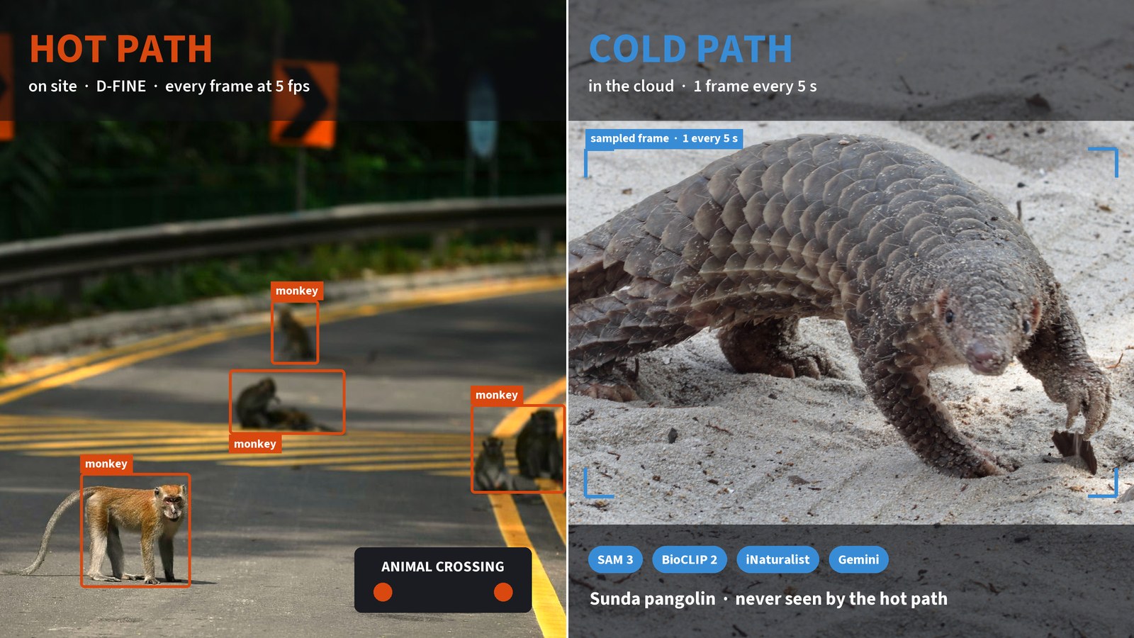
A small model can watch the road in real time, although its knowledge is limited to the data used to train it. A larger vision pipeline can recognise a wider range of wildlife, but running one on every frame from a roadside camera would be expensive and far too slow. We ended up building both and giving each one a separate job.

The fast detector on the left processes every sampled frame on site. The cloud pipeline on the right inspects one frame every five seconds and can pick up animals the detector has never seen. This is an illustration rather than real model output. Pangolin photo by Ian Dugdale, CC BY 4.0, via Wikimedia Commons.

The fast part runs beside the road

We called the real-time detector the hot path. It runs beside the camera, samples the video at five frames per second and passes each frame through D-FINE. We fine-tuned the model on footage that we labelled ourselves, including monkeys, deer and the other animals that appeared often enough for us to build a useful dataset. When it detects one of those animals, the sign lights up without waiting for an internet connection.

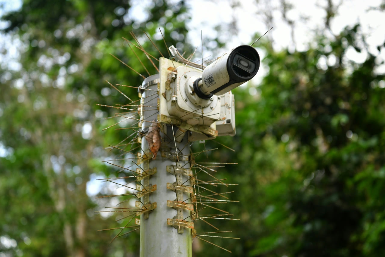
The roadside camera, complete with spikes because the local wildlife also likes sitting on it.

The detector does not need an exact species or a detailed description. Its output only has to tell us that an animal is on the road right now. In testing, it triggered for about 92% of the animals that were actually there, which I was pretty happy with.

I was less happy with the false positive rate of around 30%. Leaves moving in the wind and birds caused many of them, especially when viewed through a roadside camera at five frames per second. The cost of missing a wild boar is much higher than the cost of flashing the sign for a leaf, so some extra sensitivity made sense for this use case. It did mean that the detector’s output could not double as a reliable record of the wildlife around the road.

The slower path catches what D-FINE misses

The second system became the cold path. Every five seconds, it takes a frame regardless of what D-FINE found. A ring buffer keeps roughly ten seconds of video before and after that frame, then sends the sample to a slower cloud pipeline.

The frame goes through a few stages:

1. SAM 3 segments anything that looks like an object and produces a crop.
2. BioCLIP 2 converts each crop into an embedding.
3. A similarity search compares that embedding with species recorded in Singapore on iNaturalist.
4. Gemini receives the crop, the likely species and the surrounding video, then describes the event.
5. The result is stored in an event database for the dashboard.

While the hot path keeps the sign responsive, the cold path gives us a chance to find animals outside the detector’s training set. If a pangolin walks past, D-FINE may miss it completely, but the sampled frame can still make its way through the cloud pipeline for review.

Giving the model a sensible shortlist

My favourite part of the cold path was the combination of BioCLIP and iNaturalist. We could have sent every crop straight to a large multimodal model and asked for a species. It would usually return a confident answer, including when the image was blurry or the animal was barely visible.

We narrowed the possibilities before asking that question. BioCLIP was trained on the tree of life, so its embeddings are useful for comparing biological images. We searched those embeddings against species that had actually been recorded in Singapore on iNaturalist. Geography removed a lot of plausible-looking answers that made no sense for the camera location.

Gemini then received a short list of local candidates together with the crop and about twenty seconds of video. With that context, it could judge a manageable set of possibilities instead of naming a species from the entire animal kingdom. Splitting the work this way also let us reserve the expensive general model for the part where its reasoning and video understanding were useful.

Why we kept the surrounding video

A crop tells us what an animal looks like at one instant. The clip shows whether it crossed the road, stayed on the shoulder or lay still for the whole interval. It also helps with objects that resemble animals in a single frame. A plastic bag caught at the wrong angle can look surprisingly convincing until it starts blowing across the road.

The extra context let us store an event that someone could act on:

Species:     Long-tailed macaque
Activity:    Stationary on roadway, left shoulder
Confidence:  High
Observed:    14:32:08
Note:        No visible movement during the observed interval.
             Possible roadkill.

That is much more useful on a dashboard than a folder of crops and bounding boxes.

How a leaf made it through every model

The cold path had a failure mode that took us a while to appreciate. A bad crop could pass through the whole pipeline and come out with a detailed species description, even though none of the individual components had technically malfunctioned.

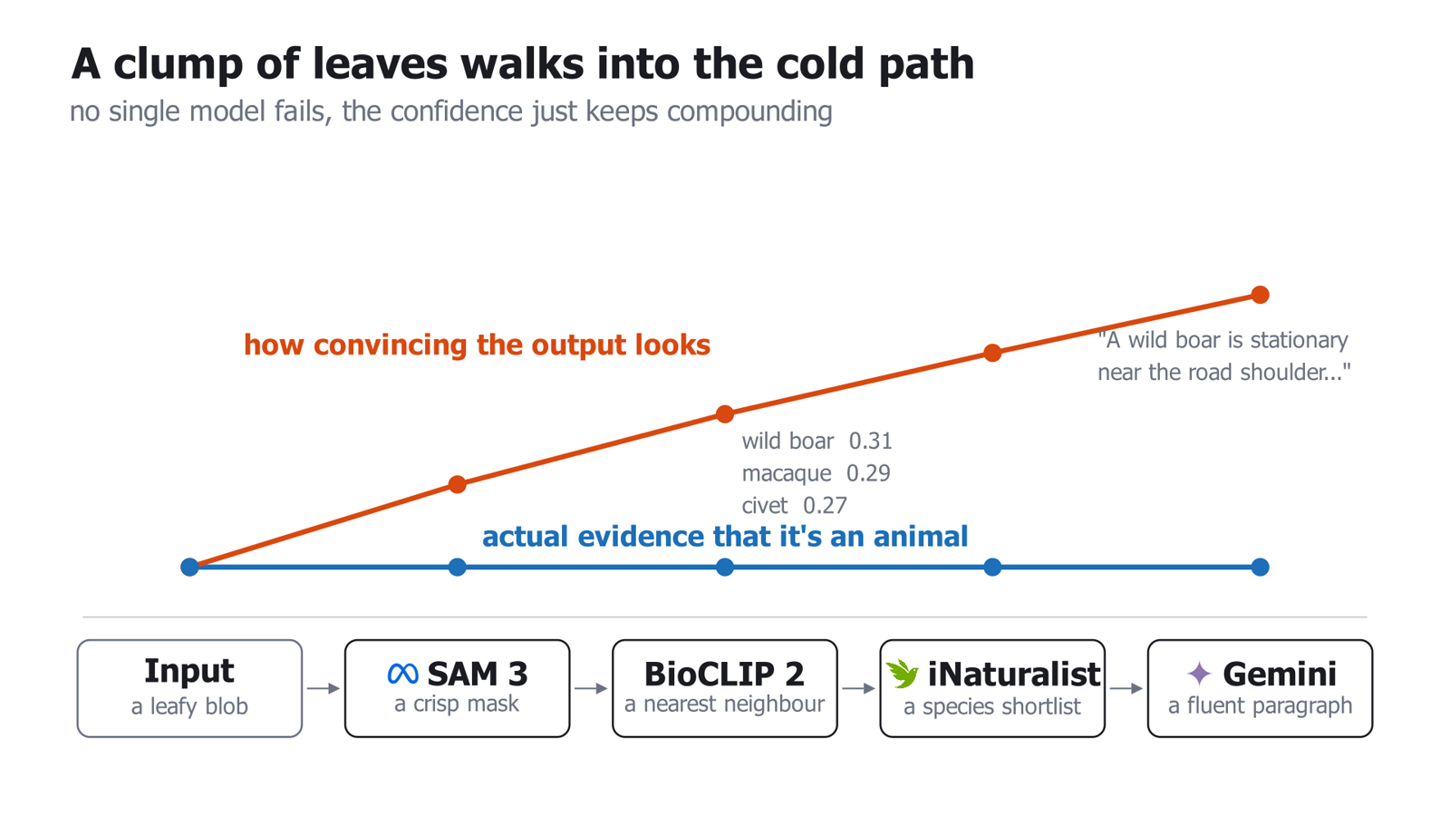
The answer becomes more polished at each stage even though the evidence has not improved.

SAM 3 can produce a very clean mask around a clump of leaves. BioCLIP will still generate an embedding for it, and a nearest-neighbour search will always return the closest entries in the index. Gemini can then write a fluent explanation based on those candidates. If the top scores are wild boar at 0.31, macaque at 0.29 and civet at 0.27, we have only learned which of three poor matches happened to be closest.

Stacking more models can make this problem harder to notice because each stage makes the result look more complete. By the time the event reaches the dashboard, the original uncertainty has been replaced by a crop, a shortlist and a paragraph that all appear to agree with one another.

We needed explicit outcomes for cases where the evidence was weak:

KNOWN SPECIES
UNKNOWN ANIMAL
NOT AN ANIMAL
NOT ENOUGH EVIDENCE

UNKNOWN ANIMAL is especially important because the cold path is supposed to discover wildlife outside the current label set. Forcing every crop onto an existing species hides those discoveries and creates bad training data. If an incorrect label is later fed back into D-FINE, the detector learns from its own mistake and produces even more of the same false positives.

Evaluating species accuracy was also difficult for a more ordinary reason: we often did not know the correct species ourselves. We are engineers, not ecologists, and a blurry snake is a fairly unforgiving test. Even with that limitation, the pipeline picked up pangolins, snakes and bronzeback tree snakes that were absent from the hot path’s training classes. Those examples were the clearest reason to keep the slower system around.

The DynamoDB table holding it together

This part of the project ate up a decent chunk of my internship. The cold path contains several slow steps spread across different cloud services, so I wanted each event to survive timeouts and partial failures. We used one DynamoDB table as a small state machine rather than putting the entire workflow into one long-running script.

Every sample gets a row with a state. Each Lambda listens for the state it handles, does one piece of work and updates the row. A DynamoDB Stream then wakes the next Lambda.

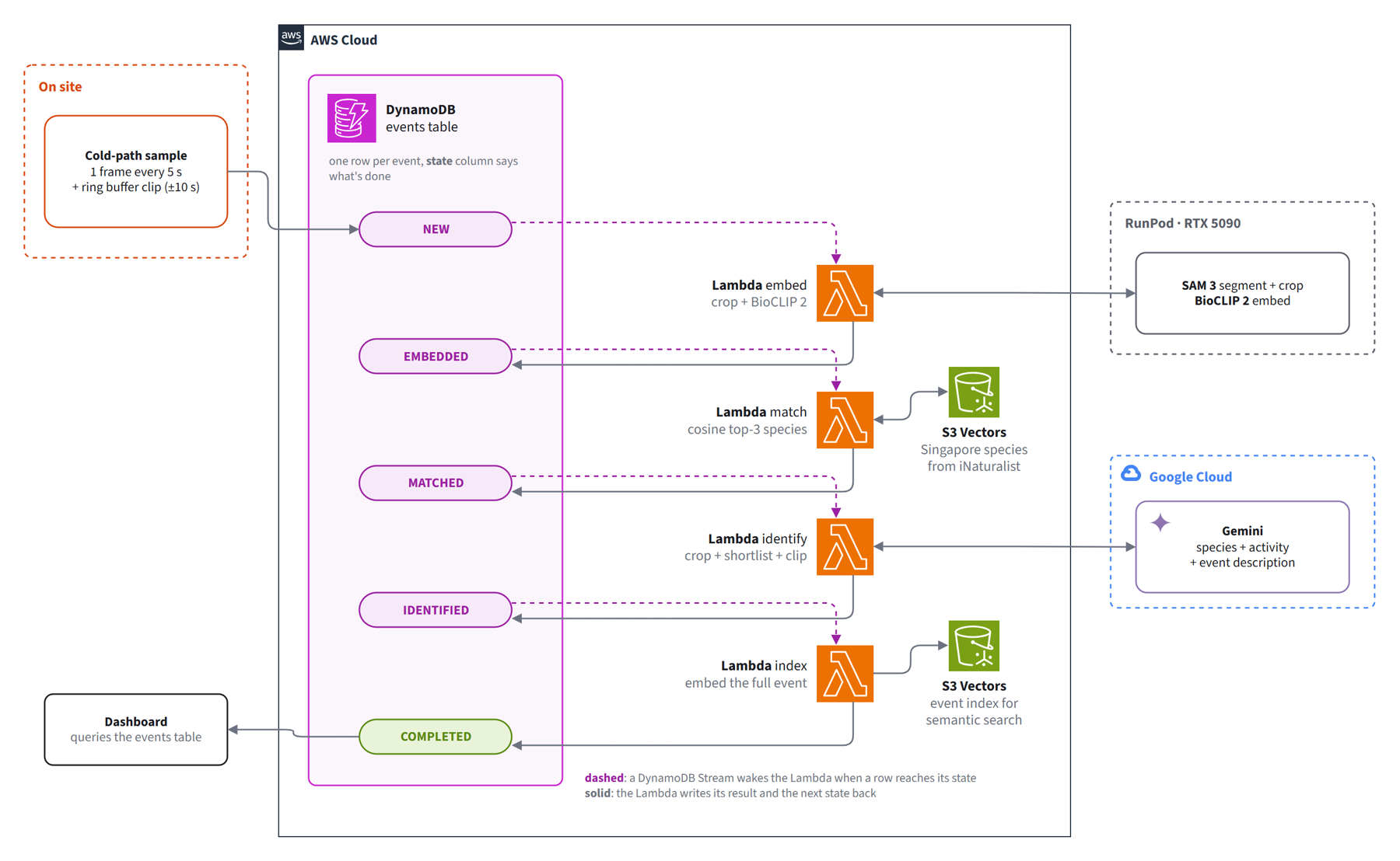
Each stage reads the event from DynamoDB, adds its result and moves it to the next state.

The workflow runs in four stages:

1. Embed. SAM 3 and BioCLIP 2 run on a RunPod RTX 5090, returning object crops and their embeddings.
2. Match. A cosine similarity search checks an S3 Vectors index built from Singapore species on iNaturalist and returns the three closest candidates.
3. Identify. Gemini receives the crop, candidates and clip, then returns the species, activity and description.
4. Index. The completed event is embedded into a second S3 Vectors index so that past events can be searched by meaning as well as species label.

Once those stages finish, the row is marked as completed and becomes available to the dashboard. If Gemini times out, the row stays at MATCHED, which shows us exactly what needs to be retried. We can also replace one model or service without changing the rest of the workflow.

I later rebuilt the cloud side on GCP as well. Doing the same project twice was painful, although it made the boundary between the actual system design and each provider’s plumbing much easier to see.

The accidental 10x speedup

When I took over the SAM 3 deployment, it was suspiciously slow for an RTX 5090. The machine had an older NVIDIA CUDA package that did not support the card, so inference had quietly fallen back to the CPU. We were paying for a top-end GPU while running the model on the processor beside it.

Updating the packages gave us roughly a 10x speedup without any changes to the model code. Since then, checking actual GPU utilisation has become one of the first things I do when an inference workload feels slower than it should.

Testing the full setup

Before handing the system over, we simulated the deployment with camera feeds exposed as RTSP streams and every stage running in its own container. We also injected latency between the roadside components and the cloud to mimic an unreliable forest connection. The pipeline held up during those tests and has since been passed to the engineering team for deployment.

Feeding the misses back into D-FINE

The next step I wanted to build was a feedback loop between the two paths. When the cloud pipeline finds an animal that D-FINE missed, a person could review the event and add the verified example to the training set. After retraining, the roadside detector would recognise the same kind of animal immediately the next time it appeared.

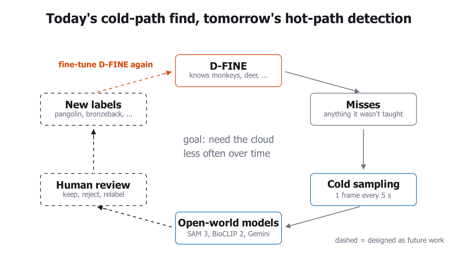
The solid arrows were implemented. The dashed arrows show the proposed feedback loop.

For a pangolin, the current route looks like this:

pangolin -> SAM 3 -> BioCLIP 2 -> iNaturalist -> Gemini -> human review

After enough verified examples and another round of training, it could become:

pangolin -> D-FINE -> sign lights up

We fine-tuned D-FINE once on our labelled footage, but the automated retraining loop was still on the roadmap when my internship ended. That was probably for the best until the uncertain cases were handled properly. Automating the feedback loop too early would allow one confident mistake to become part of the next model.

What I took away from it

The most useful decisions in this project were about scope. D-FINE had to react quickly to animals it already knew, while the cloud pipeline had more time to inspect unfamiliar cases. SAM 3, BioCLIP 2, the iNaturalist data and Gemini each handled a smaller part of that second job.

The project also changed how I think about model confidence. A result can become more polished as it moves through a pipeline without becoming more correct, especially when every component is designed to return an answer. Leaving room for uncertainty made the overall system more useful and would be essential before letting its outputs become new training data.

I also learned how to identify a bronzeback tree snake, which was nowhere in my internship expectations.

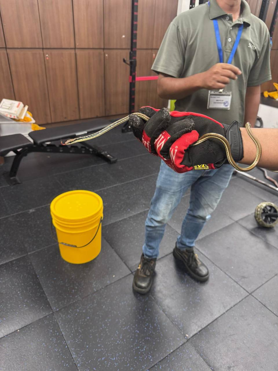
A bronzeback tree snake found at my residential college.